September 21, 2025
Have you ever tried baking a banana cake and wished you could buy tiny packets of pure sweetness or pure bitterness? Real ingredients never come that simple. Bananas bring sweetness and a little bitterness, sugar is almost all sweet, and chocolate adds sweetness with a hint of bitterness. Measuring the right amount becomes tricky, and if you just pour in 5 grams of sugar to get 5 grams of sweetness, your cake will probably be too sweet.
Math has the same problem when we try to build complicated functions out of simpler pieces. The “flavors” of math overlap, and we can easily double-count if we’re not careful. But mathematicians have a clever trick. They imagine pure, non-overlapping flavors called orthonormal bases. With the right combination of these pure flavors, you can recreate any function exactly.
In this post, we’re going to take this idea from baking to waves, look at a square wave, and use some simple math to solve a centuries-old problem. By the end, you’ll see how a messy infinite sum magically equals \(\pi^2/6\).
Imagine you want the banana cake to have exactly the right amount of sweetness, bitterness, and saltiness. In a perfect world, you could buy little jars of “pure sweetness,” “pure bitterness,” and “pure saltiness.” Sprinkle in exactly what you need, and your cake comes out perfect.
But real ingredients are messy. Bananas are sweet but a little bitter. Sugar is almost pure sweet. Chocolate adds bitterness but also a hint of sweetness. If you just pour 5 grams of sugar to get 5 grams of sweetness, your cake will probably be too sweet — because you didn’t account for the sweetness already in the bananas.
This is exactly the problem mathematicians face when they try to break a function into simpler components. If the components overlap, you can double-count some parts and miss others. You need “pure flavors” that don’t interfere with each other.
In math, these pure flavors are called orthonormal basis functions. Just like perfectly measured flavor packets in baking, each basis function contributes its own part to the function without overlapping with the others. When you mix them in the right proportions, you can recreate any function exactly.
Later, when we introduce Fourier series, think of the basis functions as these pure flavors. Each wave is a distinct flavor that doesn’t mix with the others, and the coefficients tell you exactly how much of each flavor to add. By the time we get to Parseval’s theorem, you’ll see that measuring the “power” in each wave is just like measuring how strong each flavor is in the cake (stay tuned!)
We’ve talked about pure flavors in baking — now let’s bring that idea into the world of waves. In math, our “cake” is a function, and the “flavors” are waves of different frequencies. These are called Fourier basis functions, and they let us break any periodic function into a combination of pure, non-overlapping waves.
For a function with period \(T\), the basis functions look like this:
\begin{align} \phi_n(t) &= \left\{\frac{e^{j2\pi fnt}}{\sqrt{T}}\right\}, \quad n = 0,\pm1, \pm2, \pm3, \dots \\ \end{align}
Where \(j = \sqrt{-1}\) is our imaginary number, and \(f\) is the frequency of the function, and \(f = 1/T\).
An orthonormal basis means that each basis function in the set, when projected onto itself, yields 1 (the "normal" part) and when projected onto another basis function, yields 0 (the "orthogonal" part). A projection of a signal, say \(x(t)\) onto a basis function, say \(\phi_n(t)\), is essentially measuring how much of that basis function makes up the signal. In our banana cake analogy, it's like measuring how much sweetness is there in the cake, if we "project" the cake onto the sweetness flavor.
We denote the projection of \(x(t)\) onto \(\phi_n(t)\) as \(\langle x(t), \phi_n(t) \rangle\). When \(x(t)\) is periodic with period \(T\), that projection is defined as:
\begin{align} &\langle x(t), \phi_n(t) \rangle \\ \\ =& \int_{-\frac{T}{2}} ^ {\frac{T}{2}} x(t) \phi_n^*(t)\, \mathrm{d}t \\ \end{align}
Where \(\phi_n^*(t)\) denotes the complex conjugate of \(\phi_n(t)\).
Now let's show that \(\left\{\frac{e^{j2\pi fnt}}{\sqrt{T}}\right\}\) is an orthonormal basis.
\begin{align} &\langle \phi_n(t), \phi_m(t) \rangle \\ \\ =& \int_{-\frac{T}{2}} ^ {\frac{T}{2}} \phi_n(t) \phi_m^*(t)\, \mathrm{d}t \\ \\ =& \int_{-\frac{T}{2}} ^ {\frac{T}{2}} \frac{e^{j\omega nt}}{\sqrt{T}} \frac{e^{-j\omega mt}}{\sqrt{T}}\, \mathrm{d}t \\ \\ =& \frac{1}{T}\int_{-\frac{T}{2}} ^ {\frac{T}{2}} e^{j\omega (n-m)t}\, \mathrm{d}t \\ \end{align}
Case 1: \(n = m\). In this case we have \(n - m = 0\) and so:
\begin{align} c_n &= \frac{1}{T}\int_{-\frac{T}{2}} ^ {\frac{T}{2}} e^{j\omega (n-m)t}\, \mathrm{d}t \\ \\ &= \frac{1}{T}\int_{-\frac{T}{2}} ^ {\frac{T}{2}} \, \mathrm{d}t \\ \\ &= \frac{T}{T} = 1\\ \end{align}
Case 2: \(n \neq m\). In this case we have \(n - m \neq 0\) and so:
\begin{align} c_n &= \frac{1}{T}\int_{-\frac{T}{2}} ^ {\frac{T}{2}} e^{j\omega (n-m)t}\, \mathrm{d}t \\ \\ &= \frac{1}{T}\left[\frac{e^{j\omega (n-m)t}}{j\omega (n-m)}\right]_{t = -\frac{T}{2}} ^ {t = \frac{T}{2}} \\ \\ &= \frac{1}{T}\left[\frac{e^{j\omega (n-m)(T/2)} - e^{-j\omega (n-m)(T/2)}}{j\omega (n-m)}\right] \end{align}
Recall that \(\omega = \frac{2\pi}{T}\), we have:
\begin{align} c_n &= \frac{1}{T}\left[\frac{e^{j\omega (n-m)(T/2)} - e^{-j\omega (n-m)(T/2)}}{j\omega (n-m)}\right] \\ \\ &= \frac{e^{j\pi(n-m)} - e^{-j\pi(n-m)}}{2j\pi(n-m)} \\ \\ &= \frac{\sin{[\pi (n-m)]}}{\pi (n - m)} \end{align}
Since \(n - m \neq 0\), first of all we are not dividing by zero, which is good. Second, since \(n\) and \(m\) are integers, the argument to the sine function is a multiple of \(\pi\), which means the value is always 0. This proves that:
\begin{align} \phi_n(t) &= \left\{\frac{e^{j\omega nt}}{\sqrt{T}}\right\}, \quad n = 0,\pm1, \pm2, \pm3, \dots \\ \end{align}
Is indeed an orthonormal basis to periodic signals with period \(T\).
The function \(f(t) = \frac{\sin{(\pi t)}}{\pi t}\) has a removable discontinuity at \(t = 0\), because the limit of \(f(t)\) as \(t\) approaches 0 exists and is equal to 1. When that happens, if we just assign the value \(f(0) = 1\), then we essentially make \(t = 0\) a continuous point for the function, effectively "removing" the discontinuity. When that happens, the function looks like this:
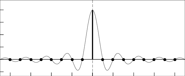
If you recognize this as the picture I placed in the "About Me" section, congratulations! I did so to reflect my proud background in signal processing. The above function, \(f(t) = \frac{\sin{(\pi t)}}{\pi t}\), is so ubiquitous in signal processing that engineers there gave it a special name, the "sinc function", pronounced as "sink". Actually, the sinc function exists in the math realm too, but engineers made two adjustments. First, the input is scaled by \(\pi\) so that the zeros of the function is always at integer values of \(t\), and second, and possibly the more egregious alternation, is that it is simply defined as:
\begin{align} \text{sinc}(t) &= \frac{\sin(\pi t)}{\pi t} \end{align}
That's it. No cases to consider, nothing. It's a function that has zeros only where \(t\) is a non-zero integer, and at \(t = 0\), it has the value of 1. This is a moment where the mathematician will object defiantly, "But the function is undefined at \(t = 0\) !". Relax, engineers know better, but by "removing" that removable discontinuity makes the expression much more efficient to, well, express. Looking at this, then we don't even need to divide our orthonormal proof from earlier into cases. Simply,
\begin{align} c_n &= \frac{1}{T}\int_{-\frac{T}{2}} ^ {\frac{T}{2}} e^{j\omega (n-m)t}\, \mathrm{d}t \\ \\ &= \text{sinc}[\pi (n - m)] \\ \\ &= \delta_{nm} \end{align}
Remember the above sinc function is a discrete-time signal with time index \((n - m)\). Since it's scaled by \(\pi\), it's value is 1 when \(n = m\) and 0 otherwise, which is exactly the definition of the Kronecker delta on the last line above. One case, no hassles.
All right, so to recap, if we have an orthonormal basis \(\{\phi_n(t)\}\) spanning the vector space of periodic signals with period \(T\), and hence \(\omega = \frac{2\pi}{T}\), our analysis equation to find how much of \(n\)th ingredient contribute to the signal \(x(t)\) in the vector space is:
\begin{align} c_n &= \int_{-\frac{T}{2}} ^ {\frac{T}{2}} x(t) \phi_n^*(t)\, \mathrm{d}t \\ \end{align}
And putting the cake together by their ingredients in the right amounts is our synthesis equation:
\begin{align} x(t) &= \sum_{n = -\infty}^{\infty} c_n \phi_n(t) \\ \end{align}
If we use the orthonormal basis that we just proved for periodic signals into \(\phi_n(t)\), we have the following equations.
Analysis equation:
\begin{align} c_n &= \frac{1}{T} \int_{-\frac{T}{2}} ^ {\frac{T}{2}} x(t) e^{-j\omega nt}\, \mathrm{d}t \\ \end{align}
Synthesis equation:
\begin{align} x(t) &= \sum_{n = -\infty}^{\infty} c_n e^{j\omega nt}\\ \end{align}
"But wait just a minute!", the mathematician once again protested passionately, "What happened to the \(\sqrt{T}\,\) in the orthonormal basis functions??? Without it, \(c_n\) are not the right ingredient amounts!"
"Calm down", the engineer replied, "we just had to make sure the basis functions are orthogonal so we don't get cross-contamination of ingredients for our cake. It's okay if the analysis equation is off by a factor of \(\sqrt{T}\), as long as the synthesis equation is off by a factor of \(1/\sqrt{T}\), which is what we have here."
"Plus", the engineer added, "by doing so, the analysis equation looks more natural, as if we are integrating over one period and dividing by the length of that period. The synthesis equation is also compact without having to carry the \(1/\sqrt{T}\) as a fraction."
*****
As a respect to the mathematicians reading my blog post, I will note that the Fourier Series works because these waves are complete, which means that if we mix the right amounts of them, we can approximate any square-integrable function as closely as we like. No flavor is left out, no note in our orchestra missing. This property makes Fourier series the perfect tool for our next step: measuring the “power” in each wave with Parseval’s theorem.
In layman terms, Parseval's Theorem equates the power of a periodic signal in time domain to that in its frequency domain, the latter being in Fourier Series form. The theorem states that:
\begin{align} \frac{1}{T}\int_{-\frac{T}{2}} ^ {\frac{T}{2}} |x(t)|^2\, \mathrm{d}t &= \sum_{n = -\infty}^{\infty}|c_n|^2 \\ \end{align}
Let's prove it!
\begin{align} \text{L.H.S} &= \frac{1}{T}\int_{-\frac{T}{2}} ^ {\frac{T}{2}} |x(t)|^2\, \mathrm{d}t \\ \\ &= \frac{1}{T}\int_{-\frac{T}{2}} ^ {\frac{T}{2}} x(t) x^*(t)\, \mathrm{d}t \\ \\ &= \frac{1}{T}\int_{-\frac{T}{2}} ^ {\frac{T}{2}} \sum_{n = -\infty}^{\infty} c_n e^{j\omega nt} \left(\sum_{n = -\infty}^{\infty} c_n e^{j\omega nt}\right)^*\, \mathrm{d}t \\ \\ &= \frac{1}{T}\int_{-\frac{T}{2}} ^ {\frac{T}{2}} \sum_{n = -\infty}^{\infty} c_n e^{j\omega nt} \sum_{n = -\infty}^{\infty} c_n^* e^{-j\omega nt}\, \mathrm{d}t \\ \\ &= \frac{1}{T}\int_{-\frac{T}{2}} ^ {\frac{T}{2}} \sum_{n = -\infty}^{\infty} \sum_{m = -\infty}^{\infty} c_n c_m^* e^{j\omega nt} e^{-j\omega mt}\, \mathrm{d}t \\ \\ &= \sum_{n = -\infty}^{\infty} \sum_{m = -\infty}^{\infty} c_n c_m^* \left[\frac{1}{T}\int_{-\frac{T}{2}} ^ {\frac{T}{2}} e^{j\omega nt} e^{-j\omega mt}\, \mathrm{d}t \right] \\ \\ &= \sum_{n = -\infty}^{\infty} \sum_{m = -\infty}^{\infty} c_n c_m^* \delta_{nm} \\ \\ &= \sum_{n = -\infty}^{\infty} c_n c_n^* \\ \\ &= \sum_{n = -\infty}^{\infty} |c_n|^2 = \text{R.H.S} \end{align}
Q.E.D.
You might notice that at one step, we swap the order of an infinite sum and an integral. In general, this isn’t always allowed — sometimes it can lead to mistakes. Luckily, in our case the function we’re working with is square-integrable, and the Fourier series converges nicely in the sense we need. That makes the swap safe.
In everyday terms, it’s like carefully measuring ingredients in a recipe: as long as each piece behaves well, we can mix them in a slightly different order without ruining the final cake. For the square wave and similar “well-behaved” functions, the math rules make this swap perfectly legal.
The following is a square wave:
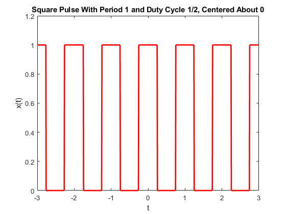
A square wave has two parameters: 1) its period, \(T\), and its duty cycle, \(\delta\), a real number between 0 and 1 describing the percentage of time in a period where the wave is "on", i.e. attaining the value of 1, vs. when it's "off", attaining the value of 0. Therefore, a square wave of period \(T\) and duty cycle \(\delta\) is the following function:
\begin{align} x(t) &= \begin{cases} 1, \quad -\frac{\delta T}{2} \leq t \leq \frac{\delta T}{2}\\ \\ 0, \quad \text{otherwise} \\ \end{cases}, \quad \text{repeats every } T \\ \end{align}
The Fourier Series coefficients of the above square wave is as follows (try to derive it using the analysis function if you are extra curious!):
\begin{align} c_n &= \begin{cases} \delta, \quad \text{if } n = 0 \\ \\ \frac{\sin(\pi n \delta)}{\pi n} , \quad \text{if } n \neq 0 \\ \end{cases} \end{align}
Which can also be succinctly written as \(c_n = \delta\, \text{sinc} (\delta n)\).
If we apply Parseval's Theorem here, we can express the power of the square wave in two ways. Let's consider \(\delta = 1/2\), i.e. a 50% duty cycle. Then, in the time domain, we have:
\begin{align} \text{Power} &= \frac{1}{T}\int_{-\frac{T}{2}} ^ {\frac{T}{2}} |x(t)|^2\, \mathrm{d}t \\ \\ &= \frac{T/2}{T} = \frac{1}{2} \\ \end{align}
In the frequency domain, we have:
\begin{align} \text{Power} &= \sum_{n = -\infty}^{\infty}|c_n|^2 \\ \\ &= \left(\frac{1}{2}\right)^2 + 2\sum_{n = 1}^{\infty} \left(\frac{\sin(\pi n/2)}{\pi n} \right)^2 \\ \\ &= \left(\frac{1}{2}\right)^2 + 2\sum_{n = 1, \, n \text{ odd}}^{\infty} \frac{1}{\pi^2 n^2} \\ \\ &= \frac{1}{4} + \frac{2}{\pi^2} \sum_{n = 1, \, n \text{ odd}}^{\infty} \frac{1}{n^2} \\ \end{align}
Equating the two equations, we have:
\begin{align} \frac{1}{2} &= \frac{1}{4} + \frac{2}{\pi^2} \sum_{k = 1}^{\infty} \frac{1}{(2k-1)^2} \\ \\ \frac{1}{4} &= \frac{2}{\pi^2} \sum_{k = 1}^{\infty} \frac{1}{(2k-1)^2} \\ \\ \frac{\pi^2}{8} &= \sum_{k = 1}^{\infty} \frac{1}{(2k-1)^2} \\ \end{align}
That is,
\begin{align} 1 + \frac{1}{3^2} + \frac{1}{5^2} + \frac{1}{7^2} + \dots &= \frac{\pi^2}{8} \\ \end{align}
The equation above by itself is already pretty neat, but we can go further. Our holy grail is \(1 + 1/2^2 + 1/3^2 + 1/4^2 + \dots\), so let's just call that value \(x\). We can see our equation from above being part of the holy grail expression, and we just have to look at the even terms in the denominator. That is:
\begin{align} &\frac{1}{2^2} + \frac{1}{4^2} + \frac{1}{6^2} + \frac{1}{8^2} + \dots \\ \\ &= \left(\frac{1}{4}\right) \left(1 + \frac{1}{2^2} + \frac{1}{3^2} + \frac{1}{4^2} + \dots \right) \\ \\ &= \left(\frac{1}{4}\right) x \end{align}
Putting everything together, we have:
\begin{align} x &= \left(\frac{1}{4}\right) x + \frac{\pi^2}{8} \\ \\ \left(\frac{3}{4}\right) x &= \frac{\pi^2}{8} \\ \\ x &= \left(\frac{\pi^2}{8}\right)\left(\frac{4}{3}\right) \\ \\ x &= \frac{\pi^2}{6} \\ \end{align}
That is,
\begin{align} 1 + \frac{1}{2^2} + \frac{1}{3^2} + \frac{1}{4^2} + \dots &= \frac{\pi^2}{6} \\ \end{align}
And there you have it: from bananas, sugar, and chocolate to waves, coefficients, and infinite sums, we’ve seen how careful measuring and pure flavors can turn chaos into something beautiful. By breaking a square wave into its “pure wave flavors” and using Parseval’s theorem, we uncovered a centuries-old secret known as the Basel problem:
\begin{align} 1 + \frac{1}{2^2} + \frac{1}{3^2} + \frac{1}{4^2} + \dots &= \frac{\pi^2}{6} \\ \end{align}
Math, like baking, is full of hidden patterns. Sometimes, the right combination of ingredients, or waves, turns a seemingly messy problem into something elegant and satisfying.