May 3, 2020
Happy May everyone! I hope everybody is staying safe and healthy during these unprecedented times. As the weather gets warmer, one might be pressed to look out the window and hear the symphony of nature, from the gentle rustling of young leaves to the crisp chirping of the robins flying about in the forest. It is during these times that make us truly appreciate how small we are compared to what mother nature has for us. I was compelled to post on Earth Day about my appreciation of the blue spaceship, of which we are her humble passengers, but due to personal matters, I have delayed posting until today. It is about nature, it is about math, and most importantly, it is about how seemingly sophisticated models that we humans create actually study things that occur routinely in nature, and those things, in turn, emerge truly sophisticated patterns.
What I am talking about (of course ;-)) is the Poisson distribution and its related Poisson process. The Poisson distribution is a discrete probability distribution related to a stochastic process called the Poisson process. If those things sound foreign to you, don't worry, I will try to make things as intuitive as possible for you later on. All you need to know, for now, is that both the distribution and the process is named after the French scientist and mathematician Simeon Denis Poisson, and both the distribution and the process are intended to model a very simple process in nature--random occurences of events of no relation to one another.
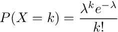
You may have learned in school the probability mass function (PMF) of the Poisson distribution. Let X be the random variable representing the number of events occurring in a unit time of rate λ, then:
Where k = 0, 1, 2, ...
(As a side note--I finally learned how to embed LaTeX into HTML, albeit in image form.)
Your initial reaction to seeing this PMF, which I might wager a buck or two, would be that of utter confusion. What you essentially have is a function comprised of an exponential multiplied by a very weird constant, and just for good measure, divided by a factorial. Who dreamed up of such an equation, and how can we expect it to model anything in the real world?
This is where the sophistication leads to simplicity. Before I continue, I would just like to introduce a few things. The first is the choose function. The function looks like the following:
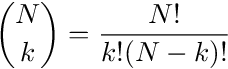
The above function reads "N choose k", where n! is the factorial function equivalent to n x (n-1) x (n-2) x ... x 1, and it represents the number of ways to arrange n items. Please note that 0! exists and is defined as 1, since there is exactly 1 way of arranging 0 items--by doing nothing!. If you have n > 0 items, there are n! ways of arranging them. For example, say you want to seat 6 people randomly in six seats. Sequentially, the first person can choose any of the six seats available, then the next person can seat anywhere from the five remaining seats, and so on, until the last peron takes the only spot left. In other words, there are 6! = 720 ways of seating 6 people. The function n! is also called a permuation function, and the arrangement of n items is called a permutation.
The choose function represents the number of ways to choose k items from a set of N items, and it is related to the permuation function in the follow way. We can think of choosing as a simplification of permutation. Imagine if we want to seat 6 people in a row of 8 chairs. Obviously in the end we will have 2 chairs left, but let's not worry about that for now. First, think about how many permutations there are in this case. The first person gets 8 choices, then the second gets 7, and so on, until the last person with three spots left. So the number of permutations is 8 x 7 x 6 x ... x 3 in this case (20160 to be exact). This is equal to 8!/(8-6)! if you think about what the factorial function is. Now, imagine if you only need to choose 6 seats for the 6 people, out of the 8 total seats. In this case, we don't really care about who seats where, just so long as six seats are boxed off out of the 8 available. In this case, we divide the previous number of permutations by the number of ways we can arrange the 6 people, i.e. 6! (if you were paying attention earlier), so that we get 8!/[6!(8-6)!], which is just (8 choose 6)--the choose function.
I plan to make a post about combinatorics later, and for now, please just remember the choose function. "N choose k" means the number of ways to choose k items among N items. Of course, it is assumed that N \(\geq\) k.
Right, so the next item I want to show you is the Binomial Distribution. Let X represent the number of successes in N trials with each trial being in no way shape or form related to other tries, and each trial having the same probability of success--let's call it p (therefore the probability of failure = (1-p)), then X has the following PMF:
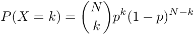
The PMF has an intuitive explanation. Since each trial is independent and identical of the others, the probability of having k successes is p^k times (1-p)^(N-k). However, we don't care which trials we succeed and which we fail, as long as there are k successes. This means that we can choose k trials among the N trials to be successful. The number of ways to do so? N choose k.
Now let's get back to topic. What does the Poisson distribution represent? What can it model in the real world? Well, in a practical sense, everything that has a random occurrence in nature in which we cannot grasp a noticeable pattern besides the rate in which it occurs--in other words: pretty much everything. Number of cars passing a busy intersection between 12pm and 1pm on a weekday? Poisson distribution. Number of customers entering a store between 10am and noon on a weekend? Poisson distribution. Number of α-particles emitted in a one-second interval by one gram of radioactive material? Definitely Poisson distribution. As long as we have a general idea of the average rate of occurrence, and we can safely assume that the occurrences are of nothing special or related to one another or any sub-intervals of the measurement duration, we can use Poisson Distrubtion to describe the number of occurrences in that duration.
The reason for the above description of the Poisson distribution lies in a very powerful assumption of nature. In the measurement interval, no matter how small, we can always divide the interval into finer and finer ones. And in a very fine interval, we can assume the following two scenarios:
I just want you to sink in the above two points for a moment, as they are essentially what the Poisson distribution is about. Imagine you work at a call center and you expect on average, 5 calls coming in per hour. Then, would it safe to say that in any given minute, the probability of receiving one call is about 5/60 or 1/12? You may say yes and no. Yes, because the calls can come in at any time during the hour and getting a call earlier means nothing in terms of when you will receive subsequent calls. But no, because it is entirely possible to receive more than one call in that minute. Okay, now I will divide the hour into 3600 second-segments. Now please repeat the exercise: would you say that the probability of receiving a call at this very literal second be 5/3600 or 1/1200? You may still say yes and no but the yes-side is gaining steam. The only thing that will make the assumption inaccurrate is the fact that you can still receive more than one call during a second time-frame, but come on, what are the chances of this happening? Nonetheless, that is the beauty of the Poisson distribution--it takes no chances. I can keep going. I am going to divide the hour into 3.6 trillion nanosecond timeframes. Yes, you heard it right, nanoseconds. Now please repeat the exercise. I would imagine you would say: yes, I expect the probability of receiving a call at this very nanosecond to be 5/3.6T, since on average I expect 5 calls per hour and there is nothing special about the way the calls arrive. The only thing that can derail that assumption is a significant chance I will be receiving two or more calls in that nanosecond timeframe, but if I do, I will quit my job and buy lotteries instead.
So there you have it. Poisson distribution models arrival events of no special pattern except for the average rate of arrival. As long as events arrive proportional to its rate throughout the measurement duration and the probability of more than one occurrence in a very small sub-interval is, practically speaking, zero, you can model the arrival event using the Poisson distribution. Thanks for reading!
Just kidding...intuition is one thing. At the end of the day, it's the math that does the talking. Let us have an arrival event with average rate of occuring be λ. In a unit time-frame, let X represent the number of occurrences. If we divide the time-frame into N sub-intervals, each interval having the probability of one arrival being λ/N and two or more being zero, then X ~ bin(N, λ/N). X would accurately represent the number of arrivals if we take N to infinity. Therefore, the probability of k arrivals in that time-frame is exactly:
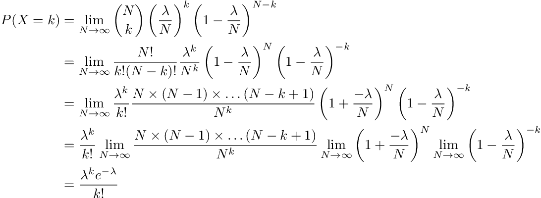
Hence, the probability corresponds to the PMF for the Poisson distribution with rate λ. I encourage readers to go over the derivation and especially with each of the limits in the last step.
The PMF of the Poisson distribution might look sophisticated, but the concept it represents is surprisingly simple.
Let us now shift gears and look at the Poisson Process. First of all, what is a stochastic process? A naive answer would be a probability function in time, but that is not entirely correct. A stochastic process, to put it plainly, is a sequence of random variables. A random variable might represent whether a toss of a coin lands heads or tails, and performing a trial realizes an occurrence of the underlying randomness of tossing the coin. In a similar fashion, a sequence of coin tosses can also be reprented by a math entity, but in this case, it is a stochastic process. Performing the sequence of coin tosses realizes an occurrence of the underlying randomness of the stochastic process, in which we call a "sample path". Unlike a random variable, however, we cannot talk about a "distribution" of a stochastic process. We can, however, either go vertical and talk about the distribution of the process at a particular index, say time, or go horizontal and talk about the relationship between successive trials in the process, or define some sample space in the process to talk about its distribution and in turn reveal something about the process. Those are the ways in which we can use stochastic processes to model real-world events.
The Poisson process is a stochastic process of the kind called "counting process". In a counting process, we have a defined time dimension t and at a particular value of t, we count the number of arrivals, N(t). Hence, N(t) for a particular value of t is a random variable, and N(t) for all t in general represents the counting process. As the name suggests, the values of N(t) must be an interger and non-decreasing. If t \(\geq\) s, then N(t) \(\geq\) N(s).
The formal definition of the Poisson process N(t) with rate λ is as follows:
The first definition is easy to follow: the counting starts at 0. The second definition means that the process is memoryless. Any arrivals in a previous time frame does not affect subsequent arrivals in the current time frame, so long as the time frames do not overlap. The third definition means that there is nothing special in the arrivals in terms of when it occurs. As long as the time-interval is fixed to be t, the number of arrivals will always be distributed in the same way, via a Poisson distribution with the corresponding rate λt.
An alternate definition of the Poisson process N(t) with rate λ is as follows in simplified language:
Does this look familiar? We again consider the arrivals in the Poisson process by looking at a very small time interval. If, we can safely assume that there are nothing special about the arrivals (captured in points 2 and 3 above), and that the probability of having one arrival is proportional to its rate, and that two or more arrivals in that small interval is practically zero, we then have ourselves a Poisson process, just like how we can decide whether a random variable has a Poisson distribution or not in the previous section.
So can a simple occurrence in nature--random arrivals with no discernable pattern except for its average rate of arrival, modeled by the Poisson process, reveal sophistications in its inner-workings? The surprising answer is yes, and one of the ways it can be obtained is by asking the following question:
What is the expected time between successive arrivals?
Yes, one thing we can study from the Poisson process, or any counting process in general, is the time between arrivals (or wait time). Wait time is an important facet of the Poisson process that reflects the nature of the arrivals. Clearly, as the arrivals are random, the wait times are random as well. Thankfully, Poisson processes are stationary, so the time between any two arrivals have the same distribution. Also thankfully, Poisson processes have independent increments, so the distribution can be determined by the time between the zeroth arrival and the first arrival, i.e. the first-arrival time. Let T be the random variable representing the wait time for the first arrival in the Poisson process.
T is a continous random variable in time. As such, to define the distribution of T, we cannot use a PMF, but instead a cumulative distribution function (CDF) instead. The CDF of a continous random variable X is defined as \(F(x) = P(X \leq x)\), i.e. the probability that X is less or equal to x. The CDF defines the distribution for its corresponding random variable.
So F(t) represents the probability that T is smaller or equal to t. In the context of how T is defined, what does it mean? It means that for a given t, up to t, we would have our first arrival. We can even have more than one arrival at time t, but at t, N(t) for sure is \(\geq\) 1. In this case, finding F(t) is not very stratightforward, so we use the indirect method. What does 1 - F(t) mean? Well, 1 - F(t) = P(T > t). This represents that for a given t, the first arrival has not yet arrived. In other words, at time t, N(t) = 0. Putting all of these together, we have, for t \(\geq\) 0:
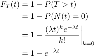
And so the CDF for the random variable T looks like the following:
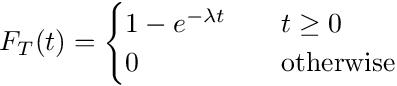
If the above looks familar to you, it is because T has an exponential distribution with parameter λ. If you are wondering how the exponential distribution is related to the Poisson process and how it came about, the above is the answer.
And here is the beauty of it all. You would think that a counting process involving events in nature seemingly mindlessly arriving with no discernable pattern to arrive in uniformly distributed times. You would think that at a call center, if we expect 5 calls per hour, then every 12 minutes we would expect a call. After all, a simple process should have simple properties, one would think. However, as the above shows, such is not the case. In a simple process where arrivals occur independently of others and are stationary throughout the process, the wait time between the arrivals is an exponential distribution, not an uniform one.
I will skip a lot of math here, but further to the sophistication we are unraveling here, I would like to show you the variance for T with parameter λ:
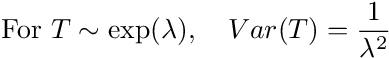
The variance of a random variable measures how likely an actual realization of it deviates from the mean (in this case the mean is 1/λ in case anyone is wondering). Remember that λ represents the average rate of arrival of the Poisson process. However, if the arrivals are not related to one another nor the time in which it occurs, the rate does not dictate that the arrival should arrive in a uniform manner. The nature of the arrivals is dependent on the rate, and as the rate gets smaller (i.e. arrivals become rarer), we will see more "clumping" or "bursts" in the process. You can try this yourself using a modeling software such as Matlab (hint: use this Matlab function). You can represent the simple Poisson process by setting a rate in which dots appear on a line or a plane and specify nothing else about how the dots appear. As time goes on, you will notice that some dots will appear to be clumped together, arrival in short intervals of one another. Other intervals will be longer. The lower you set the rate, the more likely that you will see dots clumping around one another. In this simple process, we don't observe a simple result, but rather, a sophisticated pattern of arrivals marked by clumps and large gaps.
Such phenomenon can even explain, albeit intuitively, the birthday paradox. Why is it that in a room of 23 people, we can already expect a 50% chance of two people sharing the same birthday? There are 365 days (366 if you count the leap day) in a year, so the probability of two people having the same birthday should be fairly low. However, if we imagine a process of dots landing on a date line in a year as a Poisson process (as we expect each person's birthday to be independent of that of another, especially if they are not related), then given the low rate of date clashes, we would have a large variance in the expected wait time, in this case, gaps in days between birthdays. Therefore, it would not be surprising if we already have a wait time of less than 1 day after 23 dots into the counting process.
The nature of Poisson process arrivals might be simple and without any discernable patterns, but sophistications emerge.