
January 9, 2021
Robin of Foxley has entered the FiveThirtyEight archery tournament. Her aim is excellent (relatively speaking), as she is guaranteed to hit the circular target, which has no subdivisions — it’s just one big circle. However, her arrows are equally likely to hit each location within the target.
Her true love, Marian, has issued a challenge. Robin must fire as many arrows as she can, such that each arrow is closer to the center of the target than the previous arrow. For example, if Robin fires three arrows, each closer to the center than the previous, but the fourth arrow is farther than the third, then she is done with the challenge and her score is four.
On average, what score can Robin expect to achieve in this archery challenge?
Answer: \(e\). No, not the letter, the number!
Explanation:
Solving this problem requires patiently going through steps. It's all math from here. There will be no computer simulations involved as I had pledged:
I will take a "No Simulations" challenge this time for the circle question just because it's too tempting. 😄
— David Ding (@DavidYiweiDing) January 8, 2021
So, let's begin!
Without loss of generality, let's assume the target is a unit circle (i.e with radius of 1). From the problem, it is given that Robin's arrow has an equal chance of hitting any points within the circle. In polar coordinates, let a point be \(P(R, \theta)\). How would \(R\) and \(\theta\) be distributed? We can think of the point-picking process as first choose a radius value between 0 and 1, and then on that "ring" of radius \(R\), choose an argument \(\theta\) between \(-\pi\) and \(\pi\). Clearly, given a fixed radius, all points are equally likely to be picked on a ring and so \(\theta\) is uniformly distributed between \(-\pi\) and \(\pi\). However, the radius of a circle cannot be uniform. To see why, please see the following diagram:
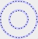
Clearly, there's more points "to be picked" as we increase the radius if all points are equally likely to be picked. Therefore, we would be more likely to pick points closer to the circle itself, i.e. points with larger radius values. We can even quantify this by using the formula for circle's circumference: \(C = 2\pi r\). Since \(\pi\) is a constant, it means that the circumference of a circle is linearly proportional to its radius, and so if \(R\) is a random variable denoting the radius of the randomly-picked point \(P\), then \(R\) would have a probability density function (pdf) of the form: \(f_R(r) = kr\), where \(k\) is some constant coefficient and \(r\) is between 0 and 1. The pdf has value of 0 otherwise. Applying the fact that the area under the pdf must be 1, we can solve for \(k\):
\begin{align} \int\limits_0^1 kr\, \mathrm{d}r &= 1 \\ \left.\frac{kr^2}{2} \right |_{r = 0}^1 &= 1 \\ \frac{k}{2} &= 1 \\ k &= 2 \end{align}
So we have: \begin{equation} f_R(r) = \begin{cases} 2r, & \quad 0 \leq r \leq 1 \\ 0, & \quad \text{otherwise} \\ \end{cases} \end{equation}
By definition: \begin{align} P(R \leq r) &= F_R(r) \\ &= \int\limits_{-\infty}^r f_R(x) \, \mathrm{d}x \\ &= \int\limits_0^r 2x \, \mathrm{d}x \\ &= \left.\frac{2x^2}{2} \right |_{x = 0}^r \\ &= r^2, \quad \text{for } 0 \leq r \leq 1 \\ \end{align}
The function \(F_R(r)\) is the cumulative density function (cdf) of the random variable \(R\), which defines the probability that the random variable is less than some value \(r\). It is also the integral of the pdf of \(R\) up to \(r\). More specifically, the cdf of \(R\) is as follows: \begin{equation} F_R(r) = \begin{cases} 0, & \quad r < 0 \\ r^2, & \quad 0 \leq r \leq 1 \\ 1, & \quad r > 1 \end{cases} \end{equation}
The cdf of \(R\), \(F_R(r)\), will come in handy later.
From the original puzzle, Robin is to shoot arrows until she shoots one that is further away from the center than the previous one. Therefore, her penultimate shot will hit a point with the minimum radius. Here let's figure out the probability that her nth shot will be the one yielding the smallest radius.
Proposition: Let \(R_n\) be the radius of the point hit by the \(n\)th shot Robin took to the circular target. The probability that \(R_n\) becomes the smallest radius, i.e. \(P(R_n \leq R_1, R_2, R_3, \dots, R_{n-1})\), is \(\frac{1}{n}\).
Intuitively, this makes sense. All \(R\)'s are independently and identically distributed (i.i.d), and so by symmetry, the probability of a particular radius being the smallest among \(n\) values would be \(\frac{1}{n}\). However, while intuition helps us reveal insights, we still need to prove our claim mathematically.
The method we use here is induction. The base case is when we only have two radius values, i.e. \(n = 2\). Here, I want to remind my readers about the total law of probability: Let \(B_1, B_2, \dots B_k\) be \(k\) mututally exclusive events whose total probability is 1, then \(P(A) = \sum_{n=1}^k P(A|B_n)P(B_n)\). If the events we are dealing with are continuous, then instead of using summation, we use integration. Therefore:
\begin{align} P(R_2 \leq R_1) &= \int\limits_0^1 P(R_2 \leq R_1 = r) f_{R_1}(r) \, \mathrm{d}r \\ &= \int\limits_0^1 F_{R_2}(r) f_{R_1}(r) \, \mathrm{d}r \\ &= \int\limits_0^1 r^2 2r \, \mathrm{d}r \\ &= \int\limits_0^1 2r^3 \, \mathrm{d}r \\ &= \left.\frac{2x^4}{4} \right |_{r = 0}^1 \\ &= \frac{1}{2} \end{align}
We have shown in the base case that \(P(R_2 \leq R_1) = \frac{1}{2}\). Let us proclaim the induction hypothesis that: \begin{equation} P(R_n \leq R_1, R_2, R_3, \dots, R_{n-1}) = \frac{1}{n} \end{equation}
Then, let us take a look at the \(n+1\) case. Here we make use of another probability identity: \(P(A, B) = P(A|B)P(B)\). \begin{align} & P(R_{n+1} \leq R_1, R_2, R_3, \dots, R_n) & \\ &= P(R_{n+1} \leq R_n | R_n \leq R_1, R_2, R_3, \dots, R_{n-1}) P(R_n \leq R_1, R_2, R_3, \dots, R_{n-1}) \\ &= P(R_{n+1} \leq R_n | R_n \leq R_1, R_2, R_3, \dots, R_{n-1}) \frac{1}{n} \\ \end{align}
Where the last line we made use of our induction hypothesis.
Nonetheless, the expression \(P(R_{n+1} \leq R_n | R_n \leq R_1, R_2, R_3, \dots, R_{n-1})\) appears to be tricky to evaluate. Before diving into the math, let's try to uncover insights by turning that expression into English. The above expression is denoting the probability that \(R_{n+1} \leq R_n\) given the fact that \(R_n\) is smaller than every other point. In other words, taking out \(R_{n+1}\), \(R_n\) is the minimum of the values \(\{R_1, R_2, \dots, R_n\}\).
So for now, let us denote \(M\) as the random variable denoting the minimum value of \(\{R_1, R_2, \dots, R_n\}\). We can determine the distribution of \(M\) by trying to ascertain its cdf, \(F_M(r)\), which by definition is:
\begin{align} F_M(r) &= P(M \leq r) \\ &= 1 - P(M > r) \\ &= 1 - P(R_1 > r, R_2 > r, \dots R_n > r) \\ &= 1 - P(R_1 > r)P(R_2 > r)\dots P(R_n > r) \\ &= 1 - (1 - F_R(r))^n \\ &= 1 - (1 - r^2)^n \quad \text{for } 0 \leq r \leq 1 \end{align}
Okay, so that was a lot to unpack here, so let me describe everything line by line. First, by definition, the cdf of a continuous random variable is the probability that the random variable is less than or equal to some value, here denoted as \(r\). Out of \(n\) radius values, as long as one of those values is less than \(r\), then \(M\) is less than \(r\) since \(M\) denotes the minimum value. Therefore, we turn the "any" condition into an "all" condition by looking at the problem from the other side: \(P(M > r)\). Now if the minimum value is greater than \(r\), it must be that all of the \(n\) radius values must be greater than \(r\). Since \(\{R_1, R_2, \dots, R_n\}\) are i.i.d, we can then separate each of the \(n\) events into independent events all having the same probability \(P(R > r)\), which is simply the inverse cdf, or \(1 - F_R(r)\). Putting everything together and we have our \(F_M(r)\). We then continue:
\begin{align} & P(R_{n+1} \leq R_1, R_2, R_3, \dots, R_n) & \\ &= P(R_{n+1} \leq R_n | R_n \leq R_1, R_2, R_3, \dots, R_{n-1}) \frac{1}{n} \\ &= P(R_{n+1} \leq M) \frac{1}{n} \\ &= \frac{1}{n} \int\limits_0^1 F_M(r) f_{R}(r) \, \mathrm{d}r \\ &= \frac{1}{n} \int\limits_0^1 (1 - (1 - r^2)^n) 2r \, \mathrm{d}r \\ &= \frac{1}{n} \frac{n}{n+1} \\ &= \frac{1}{n+1} \end{align}
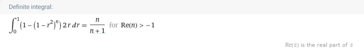
Computation courtesy of WolframAlpha.
Therefore, by the principles of mathematical induction, \(P(R_n \leq R_1, R_2, R_3, \dots, R_{n-1}) = \frac{1}{n}\). Q.E.D.
We now revisit our puzzle setup and figure out the expected score for Robin. Here we make use of a stochastic chart:
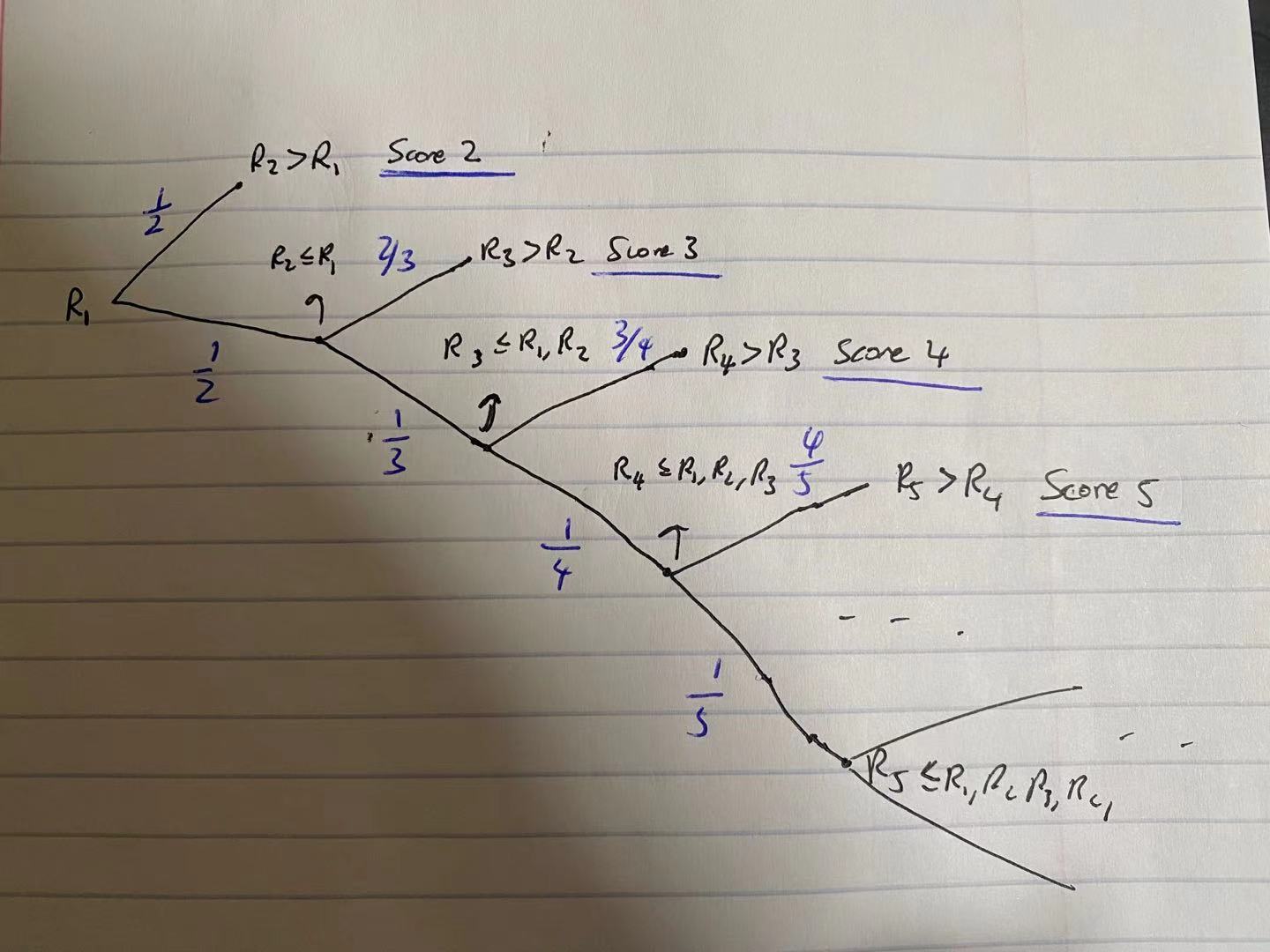
Robin takes her first shot and yields \(R_1\). Subsequently, she takes a second shot \(R_2\). If \(R_2 > R_1\), her journey ends and the final score is 2. If \(R_2 \leq R_1\), she continues firing her third shot, yielding \(R_3\). If \(R_3 > R_2\), since \(R_2 \leq R_1\), her journey is over and the final score is 3. Otherwise, if \(R_3 \leq R_1, R_2\), she continues firing until one of the \(R\)'s is greater than the minimum so far.
The probabilities written on each stochastic path comes from our proven proposition: \(P(R_n \leq R_1, R_2, R_3, \dots, R_{n-1}) = \frac{1}{n}\).
From the stochastic chart it is easy to see that for \(k = 2, 3, 4, \dots\), the probability for getting a score of \(k\) is: \begin{align} P(k) &= \frac{1}{2} \frac{1}{3} \frac{1}{4} \dots \frac{1}{k-1} \frac{k-1}{k} \\ &= \frac{1}{(k-1)!} \frac{k-1}{k} \\ &= \frac{1}{k(k-2)!} \end{align}
Hence, the expected value is:
\begin{align} \text{Expected score } &= \sum_{k=2}^\infty kp(k) \\ &= \sum_{k=2}^\infty \frac{k}{k(k-2)!} \\ &= \sum_{k=2}^\infty \frac{1}{(k-2)!} \\ &= \sum_{m}^\infty \frac{1}{m!} \\ &= e^1 \\ &= \boxed{e} \\ &\approx 2.7183 \end{align}
Here I used a change of dummy variables to let \(m = k-2\), and the infinite series is evaluated using the Taylor Series expansion for the exponential function, \(e^x\), evaluated at \(x = 1\). If you are curious, please give this a read!
Marian now uses a target with 10 concentric circles, whose radii are 1, 2, 3, etc., all the way up to 10 — the radius of the entire target. This time, Robin must fire as many arrows as she can, such that each arrow falls within a smaller concentric circle than the previous arrow. On average, what score can Robin expect to achieve in this version of the archery challenge?

Answer: Approximately 2.5585
Explanation:
Here we are taking a computer-science detour and taking dynamic programming for a spin. The strategy is to understand that once Robin has hit a ring, say ring 5, the next shot is either ring 5 or higher in which case she ends the journey, or she hits ring 1, 2, 3, or 4. Suppose we already know the expected score for those 4 rings, then the overall expectation would be either 2 shots and out or 1 shot + however many expected shots for ring 4 and lower. Dynamic programming is all about building upon previous solutions, and here we will make use of that.
Let \(p_k\) denote the probability of Robin hitting ring \(k\), and \(E_k\) be her expected score given that her first shot lands within ring \(k\) (including the first shot). Then her expected score would be:
\begin{align} \text{Expected score } &= \sum_{k=1}^{10} p_k E_k \\ \end{align}
For the p's, since inside the target all points are equally likely to be hit, the probability of hitting a ring would simply be the ratio of the area of the ring divided by the area of the entire circle (ring 1 is technically the unit circle, I know). I will leave this to the readers to show that \(p_k = \frac{2k-1}{100}\) for \(k = 1, 2, 3, \dots, 10\).
As for the E's, we will leverage dynamic program and build our solution from the center out. Starting with \(E_1\), which we know is 2 because once Robin hits the center ring, she will be out the next shot as it cannot be within the innermost circle. What about \(E_2\)? Well, if her first shot lands on ring 2, and her second shot lands on ring 2 or above, then she will still have a score of 2. When she hit ring 1 next, then her expected score would become \(E_1 + 1\). We don't care what \(E_1\) would be, rather only care about the fact that we add 1 to it because our first shot has happened outside of ring 1. When we scale each scenario by the respective probabilities, we get:
\begin{equation} E_2 = 2(1 - p_1) + p_1 (E_1 + 1) \end{equation}
Since the probability of NOT hitting ring 1 to extend the score would be \(1 - p_1\). Now we have \(E_1\) and \(E_2\), and we can use it to build upon \(E_3\):
\begin{equation} E_3 = 2(1 - p_1 - p_2) + p_1 (E_1 + 1) + p_2 (E_2 + 1) \end{equation}
And so on and so forth. When we are computing \(E_k\), we would already have the values of \(\{E_1, E_2, \dots E_{k-1}\}\). And so:
\begin{equation} E_k = 2(1 - p_1 - p_2 - \dots - p_{k-1}) + p_1 (E_1 + 1) + p_2 (E_2 + 1) + \dots p_{k-1} (E_{k-1} + 1) \end{equation}
\begin{align} \text{Expected score } &= \sum_{k=1}^{10} p_k E_k \\ \end{align}
The following is the algorithm for computing the expected score using MATLAB:
pInput = 1:10;
p = getProb(pInput); %p = (2*pInput - 1) / 100

E = NaN(1, 10);
E(1) = 2;
for k = 2:10
   E(k) = 2*(1 - sum(p(1:k-1)));
   for i = 1:k-1
      E(k) = E(k) + p(i)*(E(i) + 1);
   end
end

EFinal = sum(p.*E);
The result displayed is:
>> EFinal

EFinal =

    2.5585
Here is the various values of \(E_k\):
>> E

E =

    2.0000    2.0100    2.0403    2.0923    2.1688    2.2740    2.4141    2.5979    2.8376    3.1500
Please note: even though I used the aid of computers, it was not a simulation, but rather a computation.
It is interesting to note that the value of 2.5585 is very close to the value of \(e\) already for 10 divisions of the target. I will leave it as a challenge for my readers to show that as the number of divisions of the circular target goes to infinity (without changing the size of the target), the expected score converges to \(e\).