David Ding: Riddler Classic January 22, 2021

(The express was pretty straightforward, so I skipped the write-up for that one.)

Congratulations, you’ve made it to the finals of the Riddler Ski Federation’s winter championship! There’s just one opponent left to beat, and then the gold medal will be yours.

Each of you will complete two runs down the mountain, and the times of your runs will be added together. Whoever skis in the least overall time is the winner. Also, this being the Riddler Ski Federation, you have been presented detailed data on both you and your opponent. You are evenly matched, and both have the same normal probability distribution of finishing times for each run. And for both of you, your time on the first run is completely independent of your time on the second run.

For the first runs, your opponent goes first. Then, it’s your turn. As you cross the finish line, your coach excitedly signals to you that you were faster than your opponent. Without knowing either exact time, what’s the probability that you will still be ahead after the second run and earn your gold medal?

Without loss of generality, let \(X_1, X_2, Y_1, Y_2\) denote the random variables, all independently and identically distributed (i.i.d) \(\sim N(0, \frac{1}{2})\), that represent the times of the 1st and 2nd runs of you and your opponent, respectively. If you are feeling uneasy about the prospect of a "negative" time, then you can treat the random variables as time deviations from the course average, say. Further, let's define \(D_1 = X_1 - Y_1\), and \(D_2 = X_2 - Y_2\), i.e. the differences of the 1st and 2nd run times between you and your opponent, respectively.

Since \(X_1, X_2, Y_1, Y_2\) are independent and distributed normally, then \(D_1, D_2\) are also normally distributed. We can compute their means and variances using the basics of statistics:

\begin{align} D_1 &\sim N(0 - 0, \frac{1}{2} + (-1)^2 \frac{1}{2}) = N(0, 1) \\ D_2 &\sim N(0 - 0, \frac{1}{2} + (-1)^2 \frac{1}{2}) = N(0, 1) \\ \end{align}

Remember, for two random variables \(X, Y\), the mean of \(X \pm bY\) is simply \(\mu_X \pm b\mu_y\) and the variance is \(\sigma_X^2 + b^2 \sigma_Y^2\). If \(X, Y\) are independent and both normally distributed, then their linear combination is also normally distributed.

So now we have \(D_1\) and \(D_2\) both are i.i.d with the standard normal distribution. From the problem, we are given that \(D_1 \leq 0\) as you are ahead in the first run. What the problem is asking can be mathematically written as:

We can express the above probability using the conditional probability formula as follows: \begin{align} &P(D_1 + D_2 \leq 0 | D_1 \leq 0) & \\ &= \frac{P(D_1 + D_2 \leq 0, D_1 \leq 0)}{P(D_1 \leq 0)} \\ \end{align}

Remember, \(D_1 \sim N(0, 1)\), so it is a Gaussian curve centered and symmetric about \(x = 0\), i.e. the y-axis. Hence, \(P(D_1 \leq 0) = \frac{1}{2}\). Also, less and less or equal to here are equivalent, since we are working with continuous random variables here.

For \(P(D_1 + D_2 \leq 0, D_1 \leq 0)\), we are trying to compute the probability that the combined time differences are still less or equal to 0 while the first time difference is less or equal to 0. We can make sense of this expression by re-arranging the terms:

\begin{align} &P(D_1 + D_2 \leq 0, D_1 \leq 0) & \\ &= P(D_2 \leq -D_1, D_1 \leq 0) \\ &= P(D_2 \leq -D_1, -D_1 > 0) \end{align}

This \(-D_1\) is just another random variable, linearly transformed from \(D_1\) by a scalar multiple of -1. Hence \(-D_1\) is still normally distributed with mean \(= -1 \times 0 = 0\) and variance \(= (-1)^2 \times 1 = 1\).

Furthermore, the purpose of the above re-arranging is to express a probability of the form \(P(X \leq x)\), which we know from reading the previous Riddler solutions to be the definition for the cumulative distribution function (c.d.f) of \(X\), denoted as \(F_X(x)\). Since \(D_1, D_2, -D_1\) are all i.i.d, we let the random variable \(D \sim N(0, 1)\) represent all three of them. Hence, all three random variables have the c.d.f. \(F_D(x)\). Their corresponding probability density function (p.d.f) is the derivative of c.d.f with respect to \(x\), which is denoted as \(f_D(x)\).

The last step is to realize that whenever you have a probability of a random variable in comparison with another variable, you realize the second variable and weight it across all constrained values. In our case above, we have:

So we realize the values of \(-D_1\) and noting that we must only consider non-negative values.

\begin{align} &P(D_2 \leq -D_1, -D_1 > 0) & \\ &= \int_0^\infty P(D_2 \leq -D_1 = x, -D_1 = x) f_D(x) \mathrm{d}x \\ &= \int_0^\infty F_D(x) f_D(x) \mathrm{d}x \\ \end{align}

We only integrate from 0 to \(\infty\) instead of starting at \(-\infty\) because \(-D_1 > 0\).

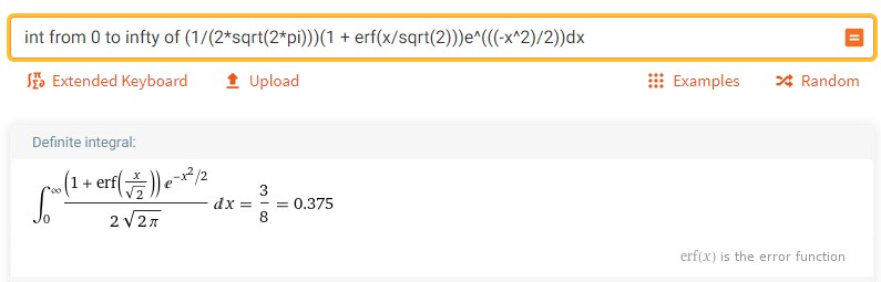
Zach has generously provided the information for the normal distribution on Wolfram, so we can write down the actual expressions for \(F_D(x)\) and \(f_D(x)\)

\begin{align} &P(D_2 \leq -D_1, -D_1 > 0) & \\ &= \int_0^\infty F_D(x) f_D(x) \mathrm{d}x \\ &= \int_0^\infty \left[\frac{1}{2}\left(1 + \text{erf}\left(\frac{x}{\sqrt{2}}\right)\right)\right] \left[\frac{e^{-\frac{x^2}{2}}}{\sqrt{2 \pi}}\right] \mathrm{d}x \\ &= \frac{3}{8} \end{align}

Where "\(\text{erf}\)" is the error function and the answer is courtesy of Wolfram Alpha:

\begin{align} &P(D_1 + D_2 \leq 0 | D_1 \leq 0) & \\ &= \frac{P(D_1 + D_2 \leq 0, D_1 \leq 0)}{P(D_1 \leq 0)} \\ &= \frac{P(D_2 \leq -D_1, -D_1 > 0)}{P(D_1 \leq 0)} \\ &= \frac{\int_0^\infty \left[\frac{1}{2}\left(1 + \text{erf}\left(\frac{x}{\sqrt{2}}\right)\right)\right] \left[\frac{e^{-\frac{x^2}{2}}}{\sqrt{2 \pi}}\right] \mathrm{d}x}{\frac{1}{2}} \\ &= \frac{3/8}{1/2} \\ &= \boxed{\frac{3}{4}} \end{align}

An intuitive interpretation of the above answer is that it is the average of two scenarios: either your lead is so large from the first run that the second run won't make a difference and you win with probability of 1, or the first run's lead is so narrow that it's still anybody's game, and so effectively the second run determines the entire result, in which case as you are evenly matched with your opponent and your winning probability becomes \(\frac{1}{2}\). The halfway point is \(\frac{3}{4}\).

Extra Credit

Over in the snowboarding championship, there are 30 finalists, including you (apparently, you’re a dual-sport threat!). Again, you are the last one to complete the first run, and your coach signals that you are in the lead. What is the probability that you’ll win gold in snowboarding?

   
function res = didFirstWinnerWin(N)
    % N is the number of participants
    firstRunTimes = randn(N, 1);
    [~, mindx1] = min(firstRunTimes);
    secondRunTimes = randn(N, 1);
    totalRunTimes = firstRunTimes + secondRunTimes;
    [~, mindx2] = min(totalRunTimes);
    
    res = mindx1 == mindx2;
end

%% main script
simCount = 1e8;
N = 30;
winCount = 0;
for k = 1:simCount
     if didFirstWinnerWin(N)
         winCount = winCount + 1;
     end
end

winProb = winCount / simCount;

>> winProb =

    0.3147

Riddler Classic: January 22, 2021

Can You Skillfully Ski The Slopes?

Extra Credit