June 10, 2022
You are trying to catch a grasshopper on a balance beam that is 1 meter long. Every time you try to catch it, it jumps to a random point along the interval between 20 centimeters left of its current position and 20 centimeters right of its current position.
If the grasshopper is within 20 centimeters of one of the edges, it will not jump off the edge. For example, if it is 10 centimeters from the left edge of the beam, then it will randomly jump to anywhere within 30 centimeters of that edge with equal probability (meaning it will be twice as likely to jump right as it is to jump left).
After many, many failed attempts to catch the grasshopper, where is it most likely to be on the beam? Where is it least likely? And what is the ratio between these respective probabilities?
Most likely: from 0.2m to 0.8m mark of the beam
Least likely: 0m and 1m marks of the beam (i.e. the edges)
Ratio of most likely to least likely: 2
Explanation:
Let's start with some simulations courtesy of MATLAB to get a sense of the puzzle.
From the puzzle, we can define a hop distribution graph by dividing the beam into \(N\) divisions, here chosen at \(N = 100\) (i.e. 1cm increments) for simplicity. Then, we simulate the grasshopper given a starting position on the beam and the number of hops that it takes.
function hopDistr = getHopDistr(startingPoint, numJumps)
    % Given the starting point (between 0 and 1), obtain the hop
    % distribution vector of the grasshopper

    numBins = 100;
    hopDistr = zeros(numBins, 1); % initialize distribution

    binIdx = getBinIdx(startingPoint, numBins);
    hopDistr(binIdx) = hopDistr(binIdx) + 1;

    % Now jump!
    prevPoint = startingPoint;

    for k = 1:numJumps
        newPoint = jump(prevPoint);
        binIdx = getBinIdx(newPoint, numBins);
        hopDistr(binIdx) = hopDistr(binIdx) + 1;
        prevPoint = newPoint;
    end
end

function idx = getBinIdx(val, numBins)
    % Helper function to convert value into bin index given number of bins.

    idx = ceil(val * numBins);
end

function newPoint = jump(prevPoint)
    % Simulates a grasshopper jump based on previous point
    jumpRangeLeft = prevPoint - min(0.2, prevPoint);
    jumpRangeRight = prevPoint + min(0.2, 1-prevPoint);

    newPoint = jumpRangeLeft + (jumpRangeRight - jumpRangeLeft)*rand;
end
The main jump logic is given in the "jump" function:
function newPoint = jump(prevPoint)
    % Simulates a grasshopper jump based on previous point
    jumpRangeLeft = prevPoint - min(0.2, prevPoint);
    jumpRangeRight = prevPoint + min(0.2, 1-prevPoint);

    newPoint = jumpRangeLeft + (jumpRangeRight - jumpRangeLeft)*rand;
end
The new point can be from the left edge of the beam up to 20cm left of the previous point, and similarly for the right side. The new point is determined within the appropriate rage via uniform distribution.
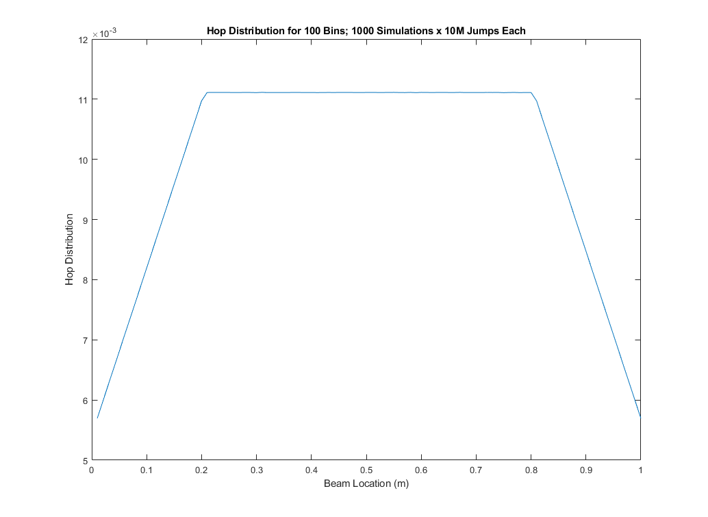
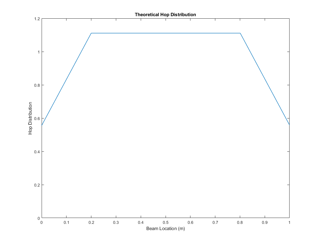
Via Monte-Carlo, 1000 different starting points are simulated, each simulation executing 10 million grasshopper jumps, to arrive at the following distribution of hops across the entire beam:
The result seems to indicate that between 0.2m and 0.8m mark of the beam, the locations are all uniformly likely. The locations tail off linearly to the edges of the beam. Let us pick some specific starting locations to see if the same result is generated.
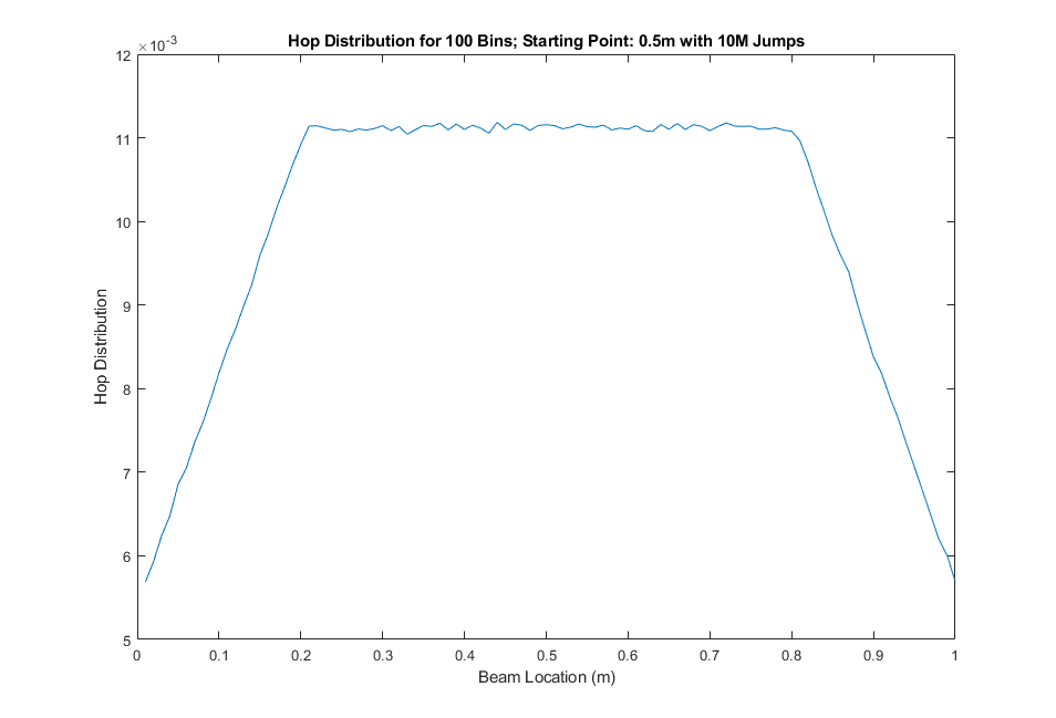
Starting point: middle of the beam (0.5m).
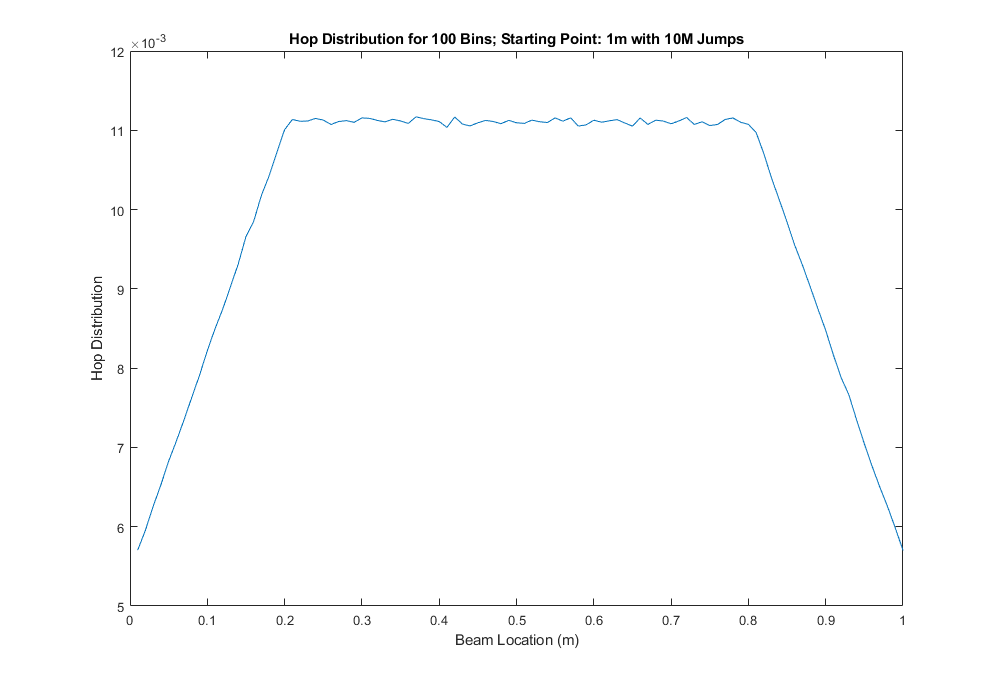
Starting point: edge of the beam (1m).
Starting point: near edge of the beam (0.1m).
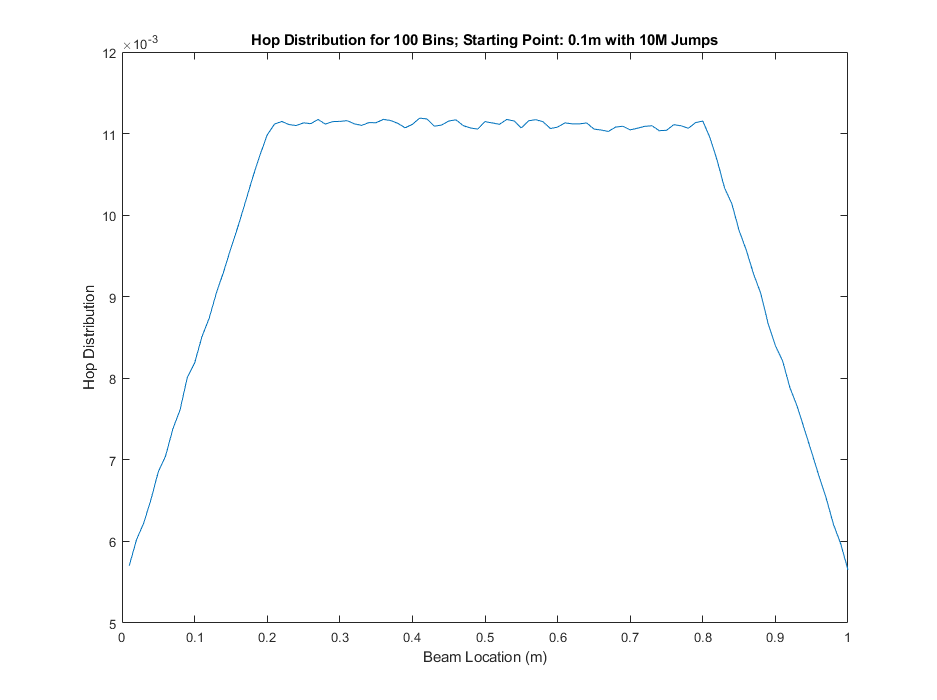
As one can see, regardless of the starting point, the grasshopper's hop distribution remains the same as the Monte-Carlo average!
From the nature of the problem, it turns out that this is similar to one of the first Riddler puzzles that I have solved regarding passing the cranberry sauce. In that puzzle, the cranberry sauce after reaching a particular guest is passed to that person's left or right with equal probability. As time goes to infinity, it turns out that everyone in the circle will have equal amount of time holding the sauce. The grasshopper performs the similar task, or one may call a "1D Random Walk".
Imagine instead we have an infinite-long beam. The grasshopper is somewhere on that beam and begins hopping within its 20cm 1D radius. We can model this as a 1D random walk by the grasshopper, where the mean is always the starting point, and every other point is equally likely to be reached as time goes to infinity. However, the beam is of finite length, and the grasshopper is "pushed" towards the middle when it gets to close to the edge. This means that between the 0.2m and 0.8m mark, the grasshoppers random walk (or should I say hop) mirrors that of the infinite beam, hence the uniform distribution seen in the Monte-Carlo result in this range. However, from the 0m to 0.2m and 0.8m to 1m ranges, the grasshopper's more likely hop is towards the center, with the odds of going to the opposite side increasing linearly as it nears the edge. This explains the trapezoidal shape of the hop distribution.
Hence, the most common place for the grasshopper to be is from 0.2m to 0.8m mark and the least common is the edge. The ratio is intuitively 2, as also confirmed by simulation results earlier. This is due to the fact that when the grasshopper is at the edge, it can only move towards the middle 0.2-0.8m range, whereas when the grasshopper is at the middle, it can move to both sides equally likely. Therefore, the probability that the grasshopper is in the middle is twice that of on the edge.
We can determine the exact distribution for the grasshopper by calculating the area of the trapezoid on a base, noting that the area under must be 1. Let \(b\) be the height of the base in which the trapezoid sits on, and \(h\) be the height of the trapezoid. Of course, we know that \(h = b\) as the most likely place (middle of the beam) is \(h + b = 2b\), and so we have:
\begin{align} 0.8h + b &= 1 \\ 0.8b + b &= 1 \\ 1.8b &= 1 \\ b &= \frac{1}{1.8} \\ \\ b &= \boxed{0.56} \\ \end{align}
This result matches with that of the simulation (scaled by the appropriate number of jumps and bins). This means the final continuous distribution of grasshopper's beam location is:
Moral of the story: wait in the middle to increase your luck catching that grasshopper!