

February 25, 2022
I have a mystery function that passes through the points (0, 1), (1, 2), (2, 4), (3, 8) and (4, 16). I also know the function is continuous and smooth. In other words, you can draw it in a single stroke without any sharp corners or cusps.
Can you find a continuous, smooth function that passes through those five points, but is decreasing at \(x = 2\)? Your answer should be an algebraic expression for the function, rather than a graph or a sketch.
One function that satisfies the conditions is: \(f(x) = -x^5 + 10.0417x^4 - 35.0833x^3 + 50.4583x^2 - 23.4167x + 1\)
Explanation:
Let's recap what is required of this function:
At first glance, it might seem impossible that a function passing through a series of "increasing" points can be decreasing along the way. The first instinct might be to resort to sinusoids, but I want to stay true to the last condition. By definition, trigonometric functions are not algebraic functions.
So what are examples of algebraic functions? Polynomials! Those classes of functions also satisfy the second condition of being continuous and smooth. If we can fit a polynomial passing through those five points, and show that it is also decreasing at \(x = 2\), then we have found a solution!
Here I want to remark on the nature of functions and calculus, a powerful tool for analyzing them--it is all about seeing the bigger picture. Just because the x and y-coordinates of five points are increasing does not mean the function itself is behaving that way. Polynomials are perfect examples of this, as the value varies greatly around \(x = 0\), but the end behavior is completely determined by its degree and the sign of its leading co-efficient. Those five measly points cannot determine the trajectory of the function itself in the grand scheme of things.
Speaking of choosing the degree of the polynomial, the ideal choice here is five degrees, balancing between the simplicity of finding its coefficients based on the five points and having enough degrees of freedom to tweak one of the coefficients to satisfy the slope requirement at \(x = 2\). The polynomial will have the following form:
\begin{align} f(x) &= a_5x^5 + a_4x^4 + a_3x^3 + a_2x^2 + a_1x + a_0 \\ \end{align}
The above polynomial has the six unknowns in the coefficients--\(a_0\) through to \(a_5\). The five equations come from plugin in the x and y-coordinates to the various \(x\)'s and their corresponding \(f(x)\)'s, respectively. Doing so yields a system of linear equations as below:
\begin{align} 1 &= a_50^5 + a_40^4 + a_30^3 + a_20^2 + a_10 + a_0 \\ 2 &= a_51^5 + a_41^4 + a_31^3 + a_21^2 + a_11 + a_0 \\ 4 &= a_52^5 + a_42^4 + a_32^3 + a_22^2 + a_12 + a_0 \\ 8 &= a_53^5 + a_43^4 + a_33^3 + a_23^2 + a_13 + a_0 \\ 16 &= a_54^5 + a_44^4 + a_34^3 + a_24^2 + a_14 + a_0 \\ \end{align}
Evaluating and writing in \(Ax = b\) form yields:
\begin{align} \begin{bmatrix} 1 & 0 & 0 & 0 & 0 & 0 \\ 1 & 1 & 1 & 1 & 1 & 1 \\ 1 & 2 & 4 & 8 & 16 & 32 \\ 1 & 3 & 9 & 27 & 81 & 243 \\ 1 & 4 & 16 & 64 & 256 & 1024 \\ \end{bmatrix} \begin{bmatrix} a_0 \\ a_1 \\ a_2 \\ a_3 \\ a_4 \\ a_5 \\ \end{bmatrix} &= \begin{bmatrix} 1 \\ 2 \\ 4 \\ 8 \\ 16 \\ \end{bmatrix} \\ \end{align}
Using the MATLAB rref function to row-reduce the augmented matrix of the above system via Gauss-Jordan Elimination yields the following result:
\begin{align} \begin{bmatrix} 1 & 0 & 0 & 0 & 0 & 0 & \bigm| & 1\\ 0 & 1 & 0 & 0 & 0 & -24 & \bigm| & 0.5833\\ 0 & 0 & 1 & 0 & 0 & 50 & \bigm| & 0.4583\\ 0 & 0 & 0 & 1 & 0 & -35 & \bigm| & -0.0833\\ 0 & 0 & 0 & 0 & 1 & 10 & \bigm| & 0.0417\\ \end{bmatrix} \\ \end{align}
Let's examine the expected output. As you might expect, for a system of five independent linear equations with six unknowns, one such unknown is denoted as a free variable. A free variable is one in which the solution can allow it to take on any value, and the other variables will take on their values based on the one chosen for the free variable. Such observation is formalized as the Rank-Nullity Theorem.
In our case, based on the way we arranged our variables in the original system of linear equations, the second-last column in the augmented matrix represents \(a_5\), and so it is the free variable here.
Therefore, the following is the general solution to the above system, in terms of the free variable \(a_5\):
\begin{align} a_0 &= 1 \\ a_1 &= 0.5833 + 24a_5 \\ a_2 &= 0.4583 - 50a_5 \\ a_3 &= -0.0833 + 35a_5 \\ a_4 &= 0.0417 - 10a_5 \\ \end{align}
How do we choose the value of \(a_5\)? That brings us to...
Now let's take the derivative of our polynomial function from earlier:
\begin{align} f(x) &= a_5x^5 + a_4x^4 + a_3x^3 + a_2x^2 + a_1x + a_0 \\ f'(x) &= 5a_5x^4 + 4a_4x^3 + 3a_3x^2 + 2a_2x + a_1 \\ \end{align}
Based on the decreasing condition, we need to have \(f(x)\) decreasing at \(x = 2\). Such condition is equivalent of saying \(f'(x = 2) < 0\). Evaluating \(x\) at this point yields the following re-written condition:
\begin{align} 80a_5 + 32a_4 + 12a_3 + 4a_2 + a_1 &< 0 \\ \end{align}
Luckily here \(a_5\) has the greatest coefficient among all terms, and therefore we can choose a relatively small negative number for it and hope that \(f'(2)\) is still less than zero. How about \(a_5 = -1\)?
\begin{align} a_0 &= 1 \\ a_1 &= 0.5833 + 24a_5 = -23.4167 \\ a_2 &= 0.4583 - 50a_5 = 50.4583 \\ a_3 &= -0.0833 + 35a_5 = -35.0833 \\ a_4 &= 0.0417 - 10a_5 = 10.0417 \\ a_5 &= -1 \\ \end{align}
Evaluating \(f'(x)\) at \(x = 2\) using the above coefficients yields \(f'(x) = -1.25 < 0\). Mission accomplished!
Therefore, one possible function is:
\begin{align} f(x) &= -x^5 + 10.0417x^4 - 35.0833x^3 + 50.4583x^2 - 23.4167x + 1 \\ \end{align}
Plotting from \(x=0\) to \(x = 4\) yields the function with the desired characteristics:
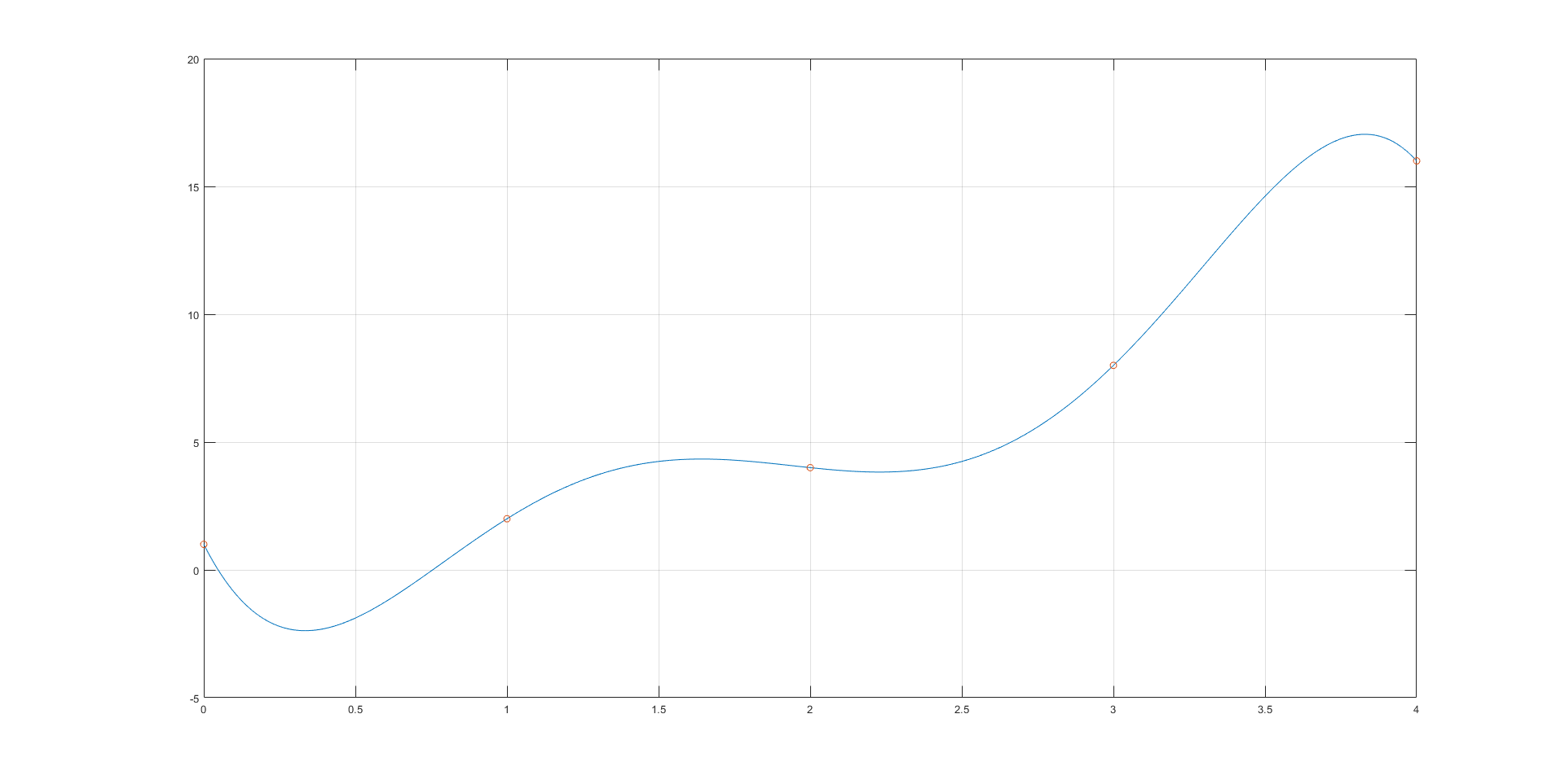
Clearly, the polynomial passes through all of the desired points. If examined more closely at around \(x=2\), the function is decreasing as it passes through (2, 4).
Echoing the point earlier to explain the seemingly counter-intuitive phenomenon that the function could be "decreasing" when it appears to be growing "exponentially": it's all about the bigger picture. Exhibit A:
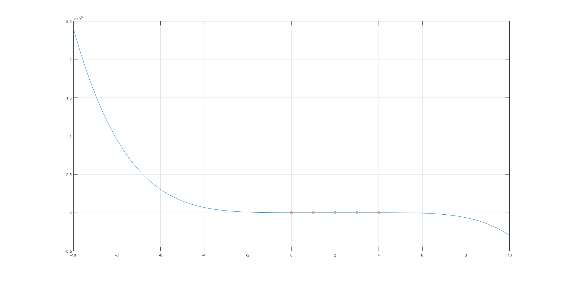
That is the same function as the one plotted for \(x=0\) to \(x=4\), except zoomed out. Here the five "exponentially growing" points that the function passes through seem to lie on a horizontal line. That is because those five points constitute the "transition" region of the polynomial, distinct from its end behavior. As the function has an odd degree with the leading coefficient being negative, the overall trend of the function is that it is decreasing, as seen in the big picture graph. When the y-axis scales up in this fashion, it is no longer surprising that the function can be decreasing at \(x=2\) while still having an "exponential growth" from 0 to 4.
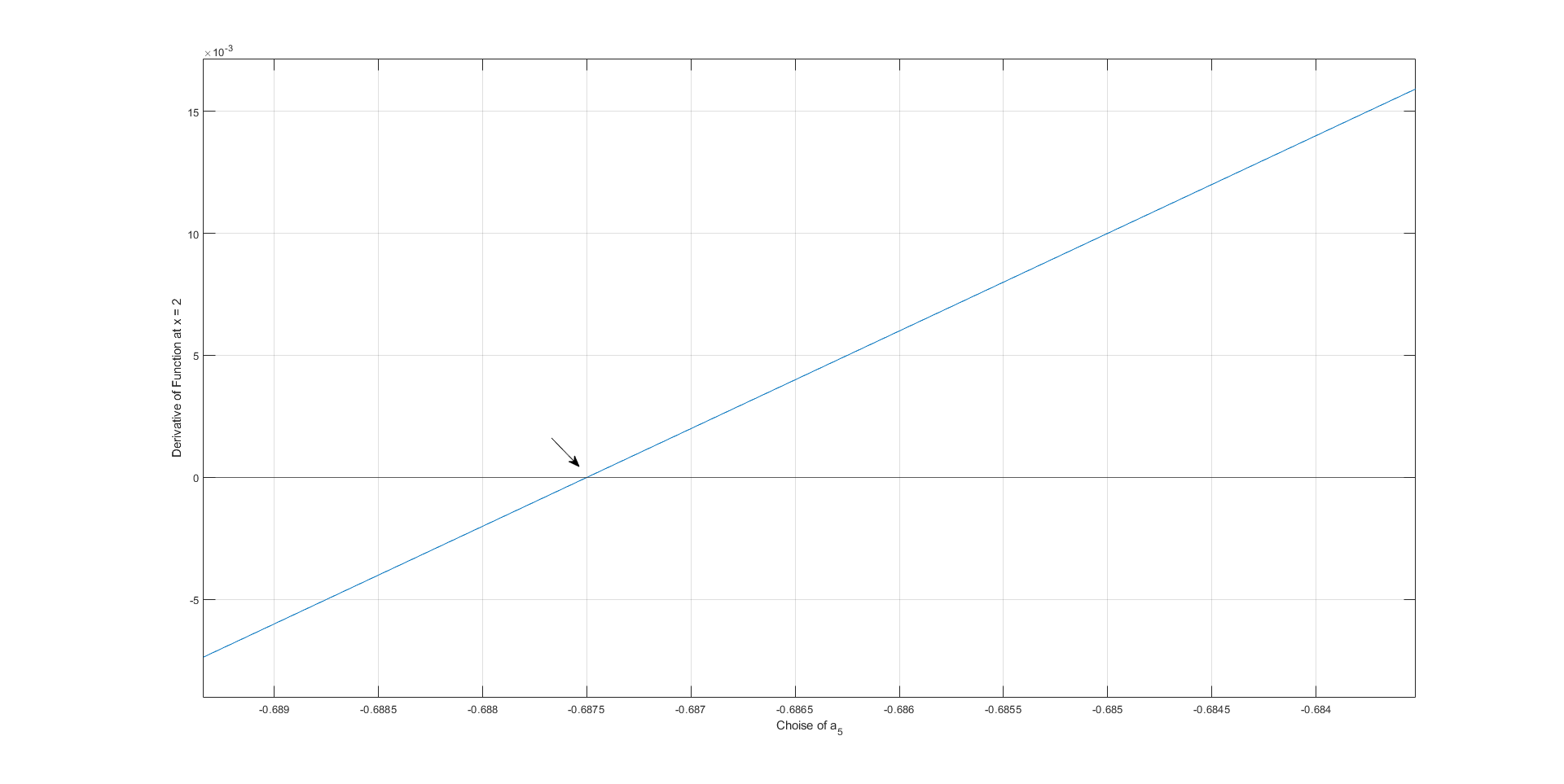
As an extension, we can find the greatest value of \(a_5\)--i.e. the least negative value such that the function is still decreasing at \(x=2\) by choosing \(a_5\) such that the derivative is zero, and therefore take a value just less than that. From an iterative search that value is close to -0.6875, yielding to a derivative of 0 at \(x=2\), as the graph below illustrates:
Plugging in \(a_5 = -0.6875\) yields the following polynomial:
\begin{align} f(x) &= -0.6875x^5 + 6.9167x^4 - 24.1458x^3 + 34.8333x^2 - 15.9167x + 1 \\ \end{align}
Plotting the above function from 0 to 4 yields:
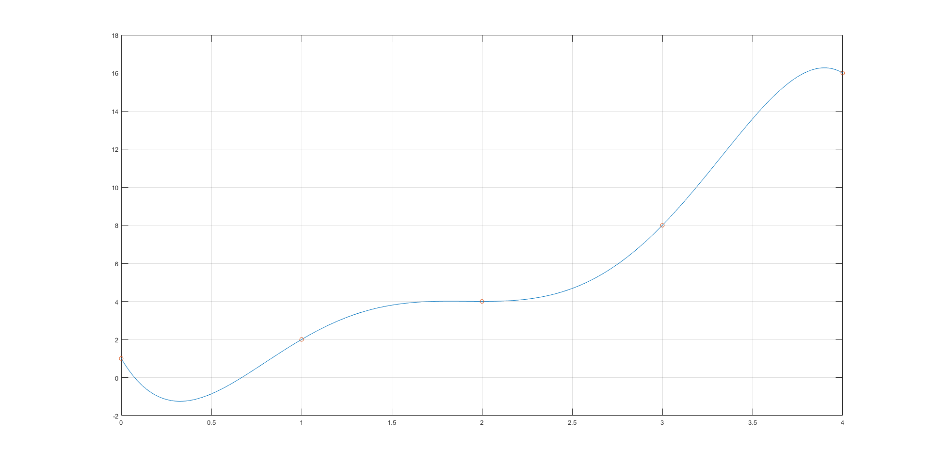
As you can see, now at \(x=2\), there is a saddle point as the derivative at that point is exactly 0. Any polynomial formed by choosing \(a_5 < -0.6785\) and other coefficients in terms of \(a_5\) will yield a function satisfying the desired conditions.